Production Line

Theory (Deeper Concepts)

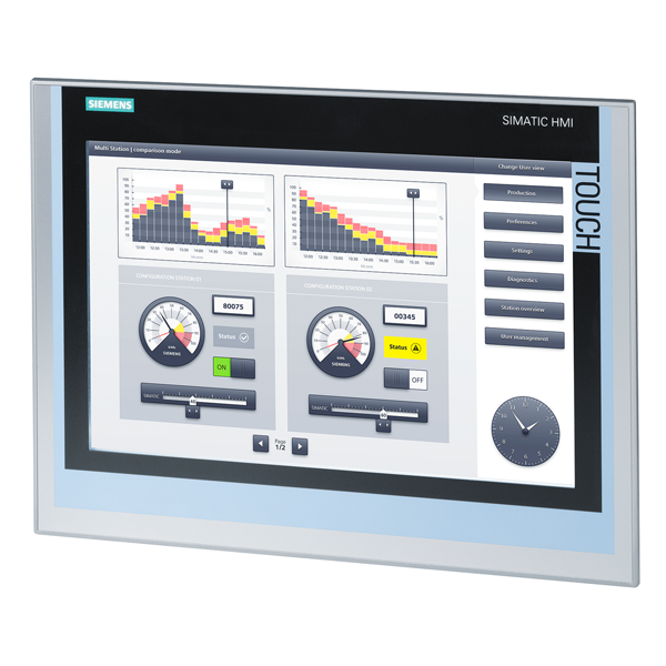
Almost every non-trivial program is split into two responsibilities. The Back End is the part the user never sees: it holds the data, runs the rules, and makes the decisions. In our case, the back end decides when a defective tip is rejected, when assembly fires, and when a pen is shipped. The Front End is the part the user sees and interacts with: text on a screen, buttons, charts, animations. Its only job is to present the back end's state and forward the user's intent back. A clean separation means the same back end can be reused with a web front end, a desktop GUI, or — as in industry — a panel mounted on a machine.

An HMI (Human-Machine Interface) is the specialized front end used in industrial automation. It is the touchscreen on a factory floor that lets an operator start the line, see how many pens have been shipped, watch live indicators turn green or red, and intervene if something fails. An HMI is not just decoration: it is the operator's window into the back end (often a PLC or SCADA system) and the operator's only safe channel to influence it. Three rules govern good HMI design: show only what the operator needs right now, make abnormal states visually unmistakable, and never let the screen lie about the state of the machine.

Mapping this to our project: ballpen_production_line.py is the Back End — pure logic, no pixels. ballpen_animation.py is the Front End, and because it visualizes a factory in real time with live counters and station status, it is essentially a small HMI. The two communicate through a shared data model (items, bins, counters), which is exactly how a real PLC publishes tags that an HMI subscribes to.

Theory (Deeper Concepts)

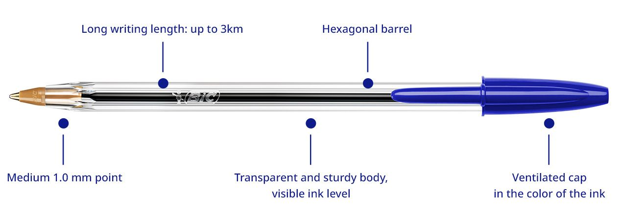
The back end models the factory as a set of cooperating objects. Dataclasses (Component, BallPen) describe what things are — plain data with a name, a serial number, and a quality. An Enum (Quality.OK, Quality.DEFECTIVE) replaces fragile string flags with values the interpreter can check. An Abstract Base Class (Station) defines the contract every workstation must honor: given an input, return an output or None. Concrete subclasses (ComponentMaker, QualityControl, AssemblyStation, FinalInspection, Packaging) each implement process in their own way.

The ProductionLine class is a composition, not an inheritance: it has stations, it does not act as one. Between QC and Assembly we keep collections.deque buffers — the software equivalent of a physical bin holding parts between machines. The orchestrator's run method is small because each part of the system has a single, well-defined responsibility — a textbook example of the Single Responsibility Principle.

Randomness simulates manufacturing variance: each maker has a defect rate (~5%) and assembly itself has a small failure rate (~2%). QC stations short-circuit defective items, returning None to signal "discard." This makes the line behave like a real one: the throughput is below the theoretical maximum, and the system must produce slightly more than the target to compensate for losses.

Theory (Deeper Concepts)

The animation is a Front End on top of the same simulation idea, written with matplotlib.animation.FuncAnimation. The fundamental pattern is the game loop: every tick we (1) clear the previous frame's transient drawings, (2) spawn new inputs, (3) advance state, (4) make decisions, and (5) render. This is the same rhythm used by every video game, every web UI library, and every industrial HMI on Earth.

Each in-flight item carries a stage field — "to_qc", "to_bin", "falling", "to_assembly" — and the renderer reads that field to decide where to draw it. This is a Finite State Machine. To synchronize the four components arriving at Assembly we use a counting semaphore (arrivals_at_assembly): when it reaches 4, we decrement by 4 and emit a finished pen. In a multithreaded version this would become an asyncio.Event or threading.Semaphore, but the logic is identical.

Crucially, the state (lists of items, bin counts, counters) is decoupled from the drawing (circles, labels, station boxes). The renderer is a pure function of the state. This is the same principle behind React, Vue, and modern HMI frameworks like Ignition or WinCC: the UI is a derivation of the data, not the source of truth. Swap matplotlib for an HTML canvas and the simulator does not change a line.

Theory (Deeper Concepts)

A Manufacturing Execution System (MES) is the software layer that sits between the shop-floor machines (PLCs, sensors, HMIs) and the enterprise business systems (ERP, supply chain). Its job is to track, coordinate, and optimize everything that happens on the factory floor in real time: which work order is running on which machine, how many good parts have been produced, where each batch of material is, and whether the line is meeting its targets right now — not tomorrow morning when someone runs a report (MES Center).

The ISA-95 standard divides factory software into four levels. Level 1 and 2 are the physical devices and control systems (sensors, PLCs, SCADA). Level 3 is the MES — it manages operations minute-to-minute. Level 4 is the ERP (SAP, Oracle) — it manages business planning day-to-week. Without the MES in between, the ERP has no live view of the factory and the machines have no awareness of production orders.

The core functions a MES provides are:

• Work order management — dispatches production orders to the right machine at the right time and tracks their progress to completion.
• Genealogy & traceability — records which materials, operators, and machines touched every unit, so a recall can be scoped to exactly the affected batch.
• Quality management — captures inline inspection results, triggers holds on suspect lots, and feeds SPC (Statistical Process Control) charts.
• Performance monitoring (OEE) — aggregates E10 machine states, cycle times, and yield data into OEE dashboards visible to operators and managers simultaneously.
• Data collection & historians — stores time-stamped process data (temperatures, pressures, speeds) that engineers mine for root-cause analysis and process improvement.

Well-known commercial MES platforms include Siemens Opcenter (formerly SIMATIC IT), Rockwell FactoryTalk, SAP ME / SAP DMC, Tulip (no-code, popular in discrete manufacturing), and Ignition by Inductive Automation (which doubles as an HMI/SCADA platform). In semiconductors, Applied Materials PROMIS and PDF Solutions Cimetrix are industry staples. Open-source options like OpenMES and Odoo Manufacturing exist for smaller operations.

The stack you build in the next section — a Python producer writing to InfluxDB, visualized in Grafana — is a miniature MES historian. It collects the same kind of time-stamped machine data that industrial historians (OSIsoft PI, InfluxDB Enterprise, Timescale) store in production at scale. The main difference is that a real MES also enforces work orders, manages operator sign-offs, and integrates with the ERP — concerns that belong above the data-collection layer you are building.

Theory (Deeper Concepts)

E10 Machine State — What It Is and Why It Matters

SEMI E10 is the semiconductor-industry standard that defines how to classify every second of a machine’s time into exactly one of six mutually exclusive states (E10 Unmasked). The three states used in our demo are:

• Productive — the machine is processing parts. This is the only state that generates revenue.
• Standby — the machine is ready but waiting for material, an operator, or a downstream station. The line is running; this machine is idle.
• Unscheduled Downtime — the machine failed unexpectedly. No parts are moving and no recovery was planned.

These states are the building blocks of OEE (Overall Equipment Effectiveness), the single most-watched KPI in manufacturing. OEE multiplies three ratios: Availability (how much of planned time the machine actually ran), Performance (how fast it ran versus its rated speed), and Quality (good parts out of total parts started). A world-class line targets OEE ≥ 85%. A machine stuck in Unscheduled Downtime drags Availability toward zero, collapsing OEE regardless of how fast or accurately the other stations run.

Tracking E10 states in a time-series database lets a plant engineer answer questions that a simple counter cannot: How long did the bottleneck spend in Standby yesterday afternoon? Did Unscheduled Downtime cluster around a shift change? Is Productive time trending up or down across the last week? These are exactly the questions Grafana’s state-timeline panel makes visible at a glance.

How the Pieces Connect

producer.py (your laptop)
      |  HTTP POST /api/v2/write   (port 8086)
      v
   InfluxDB  (Docker container)
      |  Flux queries
      v
   Grafana   (Docker container, port 3000) --> your browser

Your script never talks to Grafana directly — it only writes to InfluxDB. Grafana pulls from InfluxDB on every refresh. That decoupling is exactly the pattern used in real factories.

Step 1 — Start InfluxDB and Grafana

Save the following as docker-compose.yml in a new folder, then run docker compose up -d in that folder:

services:
  influxdb:
    image: influxdb:2.7
    container_name: influxdb
    ports: ["8086:8086"]
    environment:
      DOCKER_INFLUXDB_INIT_MODE: setup
      DOCKER_INFLUXDB_INIT_USERNAME: admin
      DOCKER_INFLUXDB_INIT_PASSWORD: admin12345
      DOCKER_INFLUXDB_INIT_ORG: lecture
      DOCKER_INFLUXDB_INIT_BUCKET: factory
      DOCKER_INFLUXDB_INIT_ADMIN_TOKEN: my-super-secret-token
    volumes: ["influx-data:/var/lib/influxdb2"]

  grafana:
    image: grafana/grafana:11.0.0
    container_name: grafana
    ports: ["3000:3000"]
    environment:
      GF_SECURITY_ADMIN_PASSWORD: admin
    depends_on: [influxdb]
    volumes: ["grafana-data:/var/lib/grafana"]

volumes:
  influx-data:
  grafana-data:

InfluxDB is now on http://localhost:8086, Grafana on http://localhost:3000 (login admin / admin).

Step 2 — Python Script That Generates Data

Install the client once:

pip install influxdb-client

Save the following as producer.py and run it with python producer.py. It prints one row per second and writes the same row to InfluxDB:

import time, math, random
from datetime import datetime, timezone
from influxdb_client import InfluxDBClient, Point
from influxdb_client.client.write_api import SYNCHRONOUS

URL    = "http://localhost:8086"
TOKEN  = "my-super-secret-token"
ORG    = "lecture"
BUCKET = "factory"

client = InfluxDBClient(url=URL, token=TOKEN, org=ORG)
write  = client.write_api(write_options=SYNCHRONOUS)

print("Sending data to InfluxDB. Ctrl+C to stop.")
t = 0
parts_total = 0
states = ["Productive", "Standby", "Unscheduled Downtime"]

try:
    while True:
        temperature = 60 + 5 * math.sin(t / 10) + random.uniform(-0.3, 0.3)
        if random.random() < 0.4:
            parts_total += 1
        state = random.choices(states, weights=[0.85, 0.10, 0.05])[0]

        point = (
            Point("machine")
            .tag("line", "A")
            .field("temperature", temperature)
            .field("parts_total", parts_total)
            .field("state", state)
            .time(datetime.now(timezone.utc))
        )
        write.write(bucket=BUCKET, record=point)
        print(f"t={t:4d}  T={temperature:5.2f}  parts={parts_total}  state={state}")
        t += 1
        time.sleep(1)
except KeyboardInterrupt:
    print("Stopped.")
finally:
    client.close()

Step 3 — Wire Grafana to InfluxDB (One-Time)

1. Open http://localhost:3000 and log in.
2. Left sidebar → Connections → Data sources → Add data source → InfluxDB.
3. Set: Query language = Flux, URL = http://influxdb:8086 (the container name, reachable inside Docker’s network), Organization = lecture, Token = my-super-secret-token, Default Bucket = factory.
4. Click Save & test — you should see “datasource is working”.

Step 4 — Build a Panel

Left sidebar → Dashboards → New → Add visualization → pick the InfluxDB datasource.

Paste this Flux query for the temperature time-series panel:

from(bucket: "factory")
  |> range(start: -5m)
  |> filter(fn: (r) => r._measurement == "machine" and r._field == "temperature")
  |> filter(fn: (r) => r.line == "A")

Hit Refresh — the line chart moves as long as producer.py is running. Set auto-refresh to 5s (top right) for a live feel.

For the parts produced panel: change the field filter to parts_total and pick the Stat visualization. For the E10 state panel: filter on state and pick the State timeline visualization.

📘 Theory (Deeper Concepts)

A Computerized Maintenance Management System (CMMS) is specialized software that tracks, schedules, and manages all maintenance activities for equipment and facilities. While a MES focuses on production execution, a CMMS focuses on keeping the machines running by orchestrating preventive maintenance, reactive repairs, spare parts inventory, and maintenance history. It is the bridge between operations and reliability engineering.

Core Functions of a CMMS

• Work order management — creates, assigns, and tracks maintenance tasks from request to completion.
• Preventive maintenance scheduling — schedules recurring maintenance (oil changes, calibrations, inspections) based on time or machine run hours to prevent failures before they happen.
• Predictive maintenance integration — ingests sensor data and alerts (temperature spikes, vibration anomalies) from the MES or historian to trigger work orders before equipment fails.
• Asset management — maintains an inventory of all equipment, their specifications, maintenance history, and genealogy.
• Spare parts tracking — manages stock levels, reorder points, and usage history to ensure critical parts are always available.
• Labor and resource planning — assigns maintenance staff, estimates task duration, and tracks labor costs per equipment.
• Root-cause analysis & reporting — documents failure modes, downtime duration, and lessons learned to drive continuous improvement.

Why CMMS Matters in Manufacturing

Unplanned downtime is the enemy of OEE. A single unexpected machine failure can halt an entire production line and cost thousands per hour. A CMMS minimizes this by shifting maintenance from reactive ("the machine broke, fix it now!") to preventive ("the machine is due for maintenance Tuesday night during the scheduled stop") or even predictive ("vibration sensors show early bearing wear; schedule maintenance before failure"). This shift improves equipment availability, extends asset life, and reduces emergency repair costs.

In the ball-pen example, SEMI E10 Scheduled Downtime is maintenance initiated by a CMMS work order. When the system knows in advance that maintenance is coming, it can pre-position materials, notify the scheduler, and avoid unexpected failures that would appear as Unscheduled Downtime — the enemy of OEE.

Popular CMMS Solutions

Commercial platforms include Maximo (IBM, enterprise-scale), SAP Plant Maintenance (PM), Infor EAM, Aspen Mtx, and Computerized Relative Allocation of Facilities (CRAFT, used in hospitals and facilities). Mid-market and discrete manufacturers often use UpKeep, Fiix (now part of IBM), or Dude Solutions. Open-source options like MINTO and OpenMAINT support smaller operations.

For more details, see OSApiens CMMS, which offers a comprehensive overview of CMMS platforms, best practices, and ROI calculations.

📘 Theory (Deeper Concepts)

In the ball-pen simulation, quality control is rule-based: each component has a Quality flag (OK or DEFECTIVE), set randomly. In a real factory, quality is measured by inspection. Historically, this meant a human operator with a magnifying glass checking for scratches, misalignment, or dimensional errors — slow, inconsistent, and prone to fatigue. Computer vision and artificial intelligence have transformed QC into a high-speed, consistent, and measurable process that runs 24/7 without tiring.

How Computer Vision and AI Work in Manufacturing QC

Computer vision is the ability of a machine to interpret images and video. A camera on the production line captures a photo of each component or assembly. Machine learning algorithms (often deep neural networks trained on thousands of examples) instantly classify the image as pass or fail, detect specific defects (cracks, discoloration, missing features), and measure dimensions with micron precision. Unlike traditional rule-based thresholds, AI models learn subtle patterns that no engineer could codify by hand.

• Defect detection — AI flags cracks, dents, stains, missing components, or misalignment in real time. The rejected item is removed automatically (by robot or diverter valve) before it reaches assembly.
• Dimensional metrology — 3D cameras or structured light systems measure part dimensions in milliseconds, comparing against CAD limits. No caliper, no subjectivity.
• Color and surface inspection — hyperspectral cameras detect coating thickness, color consistency, and surface finish anomalies that the human eye would miss.
• Traceability & genealogy — every inspected part is photographed with a timestamp and linked to the batch, operator shift, and machine that made it. A defect pattern can be traced back instantly.
• Continuous learning — as new failure modes appear, the model is retrained with fresh examples, making QC smarter over time.

Impact on OEE and Production

In our ball-pen line, the QualityControl station randomly rejects ~5% of inputs. With vision-based AI QC:

• Quality improves — recall the defect rate that reaches customers drops dramatically (from 0.5% to 0.01%) because AI catches defects that humans would miss.
• Performance stays constant — AI inspection is fast; unlike manual QC that slows the line, vision QC runs in the time it takes to snap a photo (milliseconds).
• Availability improves — fewer escaped defects means fewer customer complaints, recalls, and warranty claims. Reputation and repeat business stay intact.

Challenges and Considerations

AI QC is not magic. Challenges include: lighting and image quality must be consistent (bad photos train bad models), the model must be retrained when product design changes, rare defects are hard to learn (you need many examples), and false positives can trigger unnecessary rejections that waste parts. The solution is human-in-the-loop: controversial images are flagged for human review, with the decision fed back into model retraining. This hybrid approach combines AI speed with human judgment.

Real-World Examples

Electronics manufacturing uses AI to inspect solder joints, component placement, and circuit board traces. Automotive plants inspect painted surfaces, weld integrity, and final assembly fit. Food & beverage uses vision to sort defective products, detect foreign objects, and verify label placement. Pharmaceuticals employ vision to count pills, check seal integrity, and detect vial cracks.

For deeper insight into computer vision in manufacturing, see Tupl: Computer Vision in Manufacturing, which covers real implementations, ROI, and case studies.